Developing Drosophila (Stereo-seq)#
[26]:
import sys
sys.path.append('E:/Anaconda/envs/SpaVAEW/Lib/site-packages/')
[27]:
import glob
import numpy as np
import pandas as pd
import scanpy as sc
import matplotlib.pyplot as plt

import SpaGTL
Data loading and preprocessing#
The Stereo-seq is available at stomicsDB (https://db.cngb.org/stomics/flysta3d/). The list of marker genes can be obtained from the supplementary material of the article “High-resolution 3D spatiotemporal transcriptomic maps of developing Drosophila embryos and larvae”.
[28]:
marker=pd.read_csv("E:/data/Drosophila/Marker/STOmics_markers.csv",header=None)[0]
E16_adata=sc.read_h5ad('E:/data/Drosophila/E16-18h_a_count_normal_stereoseq.h5ad')
E16_adata.X=E16_adata.layers['raw_counts']
E16_adata=E16_adata[:,E16_adata.var_names&marker]
C:\Users\123\AppData\Local\Temp\ipykernel_5776\4275378682.py:8: FutureWarning: Index.__and__ operating as a set operation is deprecated, in the future this will be a logical operation matching Series.__and__.  Use index.intersection(other) instead.
  E16_adata=E16_adata[:,E16_adata.var_names&marker]
Spatial reconstruction#
We perform spatial reconstruction to aggregate expression from spatial neighbors.
[29]:
SpaGTL.spatial_reconstruction(E16_adata, alpha=2)
Graph Transfer Learning#
We perform graph transfer learning on the preprocessed data.
[30]:
SpaGTL.run_SpaGTL(E16_adata, n_epochs=1000)
100%|█████████████████████████████████████████████████████████████| 1000/1000 [01:21<00:00, 12.32it/s, loss: 3.971e+03]
Regulon inference and aucell#
We perform regulon inference using gene relation matrix.
[32]:
from yaml import Loader, Dumper
import glob
MOTIF_ANNOTATIONS_FNAME='E:/data/CisTarget/motifs-v9-nr.flybase-m0.001-o0.0.tbl'
tf_names=np.array((pd.read_table('E:/data/CisTarget/allTFs_dmel.txt',header=None).iloc[:,0]))
DATABASES_GLOB='E:/data/CisTarget/dm6*.feather'
db_fnames = glob.glob(DATABASES_GLOB)
SpaGTL.regulons(E16_adata, tf_names, MOTIF_ANNOTATIONS_FNAME, db_fnames, neighbors_var_key='QK')
2024-07-12 20:37:26,718 - pyscenic.utils - INFO - Creating modules.
Create regulons from a dataframe of enriched features.
Additional columns saved: []
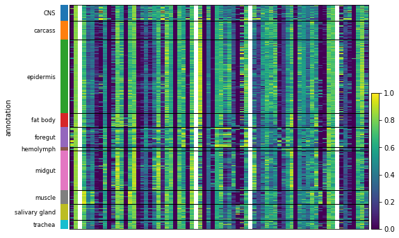
We perform aucell to compute the activity of each regulon on each spot.
[35]:
E16_adata.X=E16_adata.layers['x4']
SpaGTL.aucell(E16_adata, normalize=True)
SpaGTL.heatmap_aucell(E16_adata, E16_adata.obsm['aucell'].columns, groupby='annotation')
WARNING: Gene labels are not shown when more than 50 genes are visualized. To show gene labels set `show_gene_labels=True`
Finding differentially activity regulons#
We find the differentially activity regulons across identified domains and show the domains and their differentially activity regulons patterns in 3D spatial coordinates.
[39]:
adata_aucell = sc.AnnData(E16_adata.obsm['aucell'])
adata_aucell.obs = E16_adata.obs.copy()
adata_aucell.obsm = E16_adata.obsm.copy()
adata_aucell.obsm['spatial'] = E16_adata.obsm['spatial']
[40]:
sc.tl.rank_genes_groups(adata_aucell, groupby='annotation', method='t-test_overestim_var')
[41]:
pd.DataFrame(adata_aucell.uns['rank_genes_groups']['names']).iloc[:10,:]
[41]:
| CNS | carcass | epidermis | fat body | foregut | hemolymph | midgut | muscle | salivary gland | trachea | |
|---|---|---|---|---|---|---|---|---|---|---|
| 0 | trv(+) | oc(+) | grh(+) | srp(+) | B-H1(+) | bin(+) | sug(+) | ss(+) | jim(+) | Hey(+) |
| 1 | Sp1(+) | vvl(+) | en(+) | Ets98B(+) | SoxN(+) | peb(+) | Pdp1(+) | CG7101(+) | btd(+) | Mef2(+) |
| 2 | D(+) | en(+) | gcm2(+) | Hey(+) | pb(+) | maf-S(+) | maf-S(+) | Cf2(+) | bs(+) | bap(+) |
| 3 | fd59A(+) | ovo(+) | vvl(+) | pnt(+) | fd96Cb(+) | pnr(+) | grn(+) | Mef2(+) | SoxN(+) | CG7101(+) |
| 4 | ara(+) | sr(+) | knrl(+) | Max(+) | toy(+) | Pdp1(+) | bin(+) | bs(+) | Cf2(+) | svp(+) |
| 5 | Rfx(+) | bap(+) | slp1(+) | pnr(+) | pnr(+) | Rfx(+) | TFAM(+) | CTCF(+) | CG7101(+) | HLH54F(+) |
| 6 | zfh1(+) | Mef2(+) | sr(+) | grn(+) | btd(+) | SoxN(+) | HLH54F(+) | cyc(+) | toy(+) | ss(+) |
| 7 | ct(+) | slp1(+) | ovo(+) | TFAM(+) | sqz(+) | E2f2(+) | pnt(+) | sr(+) | fd59A(+) | TFAM(+) |
| 8 | Rbp6(+) | HLH54F(+) | bap(+) | BEAF-32(+) | svp(+) | CrebA(+) | Stat92E(+) | zfh1(+) | pb(+) | nau(+) |
| 9 | CrebA(+) | cyc(+) | ken(+) | svp(+) | E2f2(+) | BEAF-32(+) | BEAF-32(+) | Hey(+) | zfh1(+) | pnt(+) |
Here, we’ve created an interactive visualization window.
[42]:
%matplotlib notebook
%matplotlib auto
Using matplotlib backend: nbAgg
We assign a color to each spot to distinguish the spatial domain.
[43]:
def assign_colors(elements, color_map):
    """
    Assign colors to elements based on a predefined mapping.

    Parameters:
    - elements (list): List of elements to assign colors to.
    - color_map (dict): Dictionary mapping elements to their corresponding colors.

    Returns:
    - list: A list containing the colors assigned to each element.
    """
    colors = []
    # Iterate over the list of elements
    for element in elements:
        # Append the corresponding color from the color map
        if element in color_map:
            colors.append(color_map[element])
        else:
            colors.append('unknown')  # Default color if the element is not in the map

    return colors

elements = list(E16_adata.obs['annotation'])
color_map = {'CNS':'#7a4900',
 'amnioserosa':'#ffff00',
 'carcass':'#0000a6',
 'epidermis':'#FFBE7A',
 'epidermis/CNS':'#997d87',
 'fat body':'#008941',
 'fat body/trachea':'#1ce6ff',
 'foregut':'#63ffac',
 'foregut/garland cells':'#ff4a46',
 'hemolymph':'#ffdbe5',
 'hindgut':'#006fa6',
 'hindgut/malpighian tubule':'#8fb0ff',
 'midgut':'#ff34ff',
 'midgut/malpighian tubules':'#b79762',
 'muscle':'#004d43',
 'salivary gland':'#a30059',
 'testis':'#FA7F6F',
 'trachea':'#82B0D2'}

colors = assign_colors(elements, color_map)
Next, we show the spatial domain on 3D coordinates.
[48]:
fig = plt.figure(figsize=(10,10))
ax3d = fig.add_subplot(111, projection='3d')
ax3d.scatter(E16_adata.obsm['spatial'][:,0], E16_adata.obsm['spatial'][:,1], E16_adata.obsm['spatial'][:,2],s = 150, c = colors, alpha =1)

[48]:
<mpl_toolkits.mplot3d.art3d.Path3DCollection at 0x2acd8f85850>
Similarly, regulon activity can also be displayed on 3D coordinates.
[92]:
#fig = plt.figure(figsize=(10,10))
#ax3d = fig.add_subplot(111, projection='3d')
#ax3d.scatter(E16_adata.obsm['spatial'][:,0], E16_adata.obsm['spatial'][:,1], E16_adata.obsm['spatial'][:,2],s = 150, c = E16_adata.obsm['aucell']['grh(+)'], alpha =1)
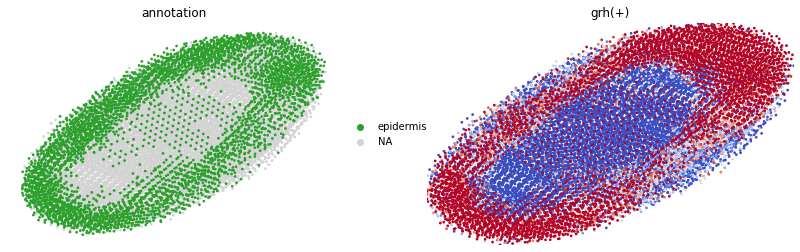
To better observe the region control pattern, we mapped 3D coordinates to 2D coordinates.
[70]:
%matplotlib inline
[71]:
coord=pd.DataFrame(adata_aucell.obsm['spatial'])
adata_aucell.obsm['spatial'] = np.matmul(coord.iloc[:,[0,1]].to_numpy(),[[np.cos(45), -np.sin(45)],[np.sin(45), np.cos(45)]])
sc.pp.scale(adata_aucell)
adata_aucell.X = np.clip(adata_aucell.X, a_min=-2.5, a_max=2.5)
[85]:
sc.pl.embedding(
                 adata_aucell,
                 basis='spatial',
                 color=['annotation','grh(+)'],
                 size=30,
                 colorbar_loc=None,
                 frameon=False,
                 vmin='p50',
                 vmax='p70',
                 cmap='coolwarm',
                 show=False,
                 groups='epidermis'
                    )
axs.set_aspect('equal')
axs.invert_xaxis()
plt.xlim([np.min(adata_aucell.obsm['spatial'], axis=0)[0], np.max(adata_aucell.obsm['spatial'], axis=0)[0]])
plt.ylim([np.min(adata_aucell.obsm['spatial'], axis=0)[1], np.max(adata_aucell.obsm['spatial'], axis=0)[1]])
plt.tight_layout()
E:\Anaconda\envs\sparcl\lib\site-packages\scanpy\plotting\_tools\scatterplots.py:392: UserWarning: No data for colormapping provided via 'c'. Parameters 'cmap' will be ignored
  cax = scatter(
C:\Users\123\AppData\Local\Temp\ipykernel_5776\23697629.py:18: UserWarning: This figure includes Axes that are not compatible with tight_layout, so results might be incorrect.
  plt.tight_layout()
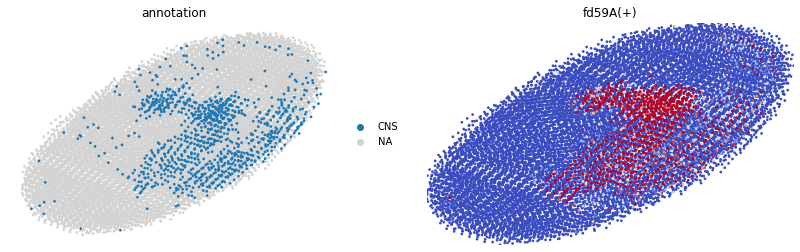
[95]:
sc.pl.embedding(
                 adata_aucell,
                 basis='spatial',
                 color=['annotation','fd59A(+)'],
                 size=30,
                 colorbar_loc=None,
                 frameon=False,
                 vmin='p90',
                 vmax='p95',
                 cmap='coolwarm',
                 show=False,
                 groups='CNS'
                    )
axs.set_aspect('equal')
axs.invert_xaxis()
plt.xlim([np.min(adata_aucell.obsm['spatial'], axis=0)[0], np.max(adata_aucell.obsm['spatial'], axis=0)[0]])
plt.ylim([np.min(adata_aucell.obsm['spatial'], axis=0)[1], np.max(adata_aucell.obsm['spatial'], axis=0)[1]])
plt.tight_layout()
E:\Anaconda\envs\sparcl\lib\site-packages\scanpy\plotting\_tools\scatterplots.py:392: UserWarning: No data for colormapping provided via 'c'. Parameters 'cmap' will be ignored
  cax = scatter(
C:\Users\123\AppData\Local\Temp\ipykernel_5776\30137340.py:18: UserWarning: This figure includes Axes that are not compatible with tight_layout, so results might be incorrect.
  plt.tight_layout()
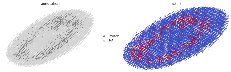
[96]:
sc.pl.embedding(
                 adata_aucell,
                 basis='spatial',
                 color=['annotation','ss(+)'],
                 size=30,
                 colorbar_loc=None,
                 frameon=False,
                 vmin='p90',
                 vmax='p95',
                 cmap='coolwarm',
                 show=False,
                 groups='muscle'
                    )
axs.set_aspect('equal')
axs.invert_xaxis()
plt.xlim([np.min(adata_aucell.obsm['spatial'], axis=0)[0], np.max(adata_aucell.obsm['spatial'], axis=0)[0]])
plt.ylim([np.min(adata_aucell.obsm['spatial'], axis=0)[1], np.max(adata_aucell.obsm['spatial'], axis=0)[1]])
plt.tight_layout()
E:\Anaconda\envs\sparcl\lib\site-packages\scanpy\plotting\_tools\scatterplots.py:392: UserWarning: No data for colormapping provided via 'c'. Parameters 'cmap' will be ignored
  cax = scatter(
C:\Users\123\AppData\Local\Temp\ipykernel_5776\3742951034.py:18: UserWarning: This figure includes Axes that are not compatible with tight_layout, so results might be incorrect.
  plt.tight_layout()