Mouse Brain (10x Visium)#
[50]:
import sys
sys.path.append('E:/Anaconda/envs/SpaVAEW/Lib/site-packages/')
import glob
import numpy as np
import pandas as pd
import scanpy as sc
import matplotlib.pyplot as plt

import SpaGTL
Data loading and preprocessing#
The datasets are available at 10x genomics website.We load the dataset and perform preprocessing including finding top 2000 highly variable genes and log transformation.
[51]:
adata = sc.read_h5ad('E:/data/Mouse_brain/V1_Adult_Mouse_Brain.h5ad')
E:\Anaconda\envs\sparcl\lib\site-packages\anndata\_core\anndata.py:1832: UserWarning: Variable names are not unique. To make them unique, call `.var_names_make_unique`.
  utils.warn_names_duplicates("var")
[52]:
adata.var_names_make_unique()
sc.pp.filter_genes(adata, min_cells=15)
sc.pp.highly_variable_genes(adata, n_top_genes=2000, flavor='seurat_v3')
adata = adata[:, adata.var['highly_variable']]
sc.pp.log1p(adata)
E:\Anaconda\envs\sparcl\lib\site-packages\scanpy\preprocessing\_simple.py:373: UserWarning: Received a view of an AnnData. Making a copy.
  view_to_actual(adata)
Graph Transfer Learning#
We perform graph transfer learning on the preprocessed data.
[53]:
params_dict = np.load('E:/data/params_dict.npy', allow_pickle=True).item()
intersection = [value for value in params_dict['genes'] if value in adata.var_names]
len(intersection)
adata=adata[:,intersection]
SpaGTL.run_SpaGTL(adata, n_epochs=1000)
100%|█████████████████████████████████████████████████████████████| 1000/1000 [00:15<00:00, 62.87it/s, loss: 1.793e+03]
E:\Anaconda/envs/SpaVAEW/Lib/site-packages\SpaGTL\_SpaGTL.py:156: ImplicitModificationWarning: Trying to modify attribute `._uns` of view, initializing view as actual.
  adata.uns[key_added] = {}
E:\Anaconda\envs\sparcl\lib\site-packages\anndata\_core\anndata.py:1832: UserWarning: Variable names are not unique. To make them unique, call `.var_names_make_unique`.
  utils.warn_names_duplicates("var")
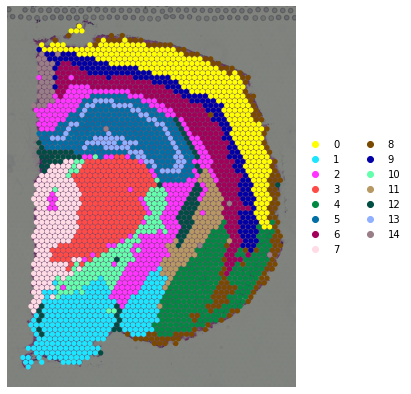
Spatial domain identification#
We identify spatial domians using the relation matrix.
[57]:
#sc.pp.neighbors(adata, use_rep='qz')
#sc.tl.leiden(adata, resolution=1)
#adata.obs['leiden'].to_csv('./leiden.csv')
c=pd.read_csv('./leiden.csv',index_col=0)
adata.obs['leiden']=c['leiden'].astype('category')
fig, axs = plt.subplots(figsize=(7, 7))
sc.pl.spatial(
    adata,
    img_key='hires',
    color='leiden',
    size=1.5,
    palette=sc.pl.palettes.default_102,
    legend_loc='right margin',
    frameon=False,
    title='',
    show=False,
    ax=axs,
)
[57]:
[<AxesSubplot: xlabel='spatial1', ylabel='spatial2'>]
Regulon inference and aucell#
We perform regulon inference using gene relation matrix.
[59]:
from yaml import Loader, Dumper
import glob
MOTIF_ANNOTATIONS_FNAME='E:/data/CisTarget/motifs-v9-nr.mgi-m0.001-o0.0.tbl'
tf_names=np.array((pd.read_table('E:/data/CisTarget/mm_mgi_tfs.txt',header=None).iloc[:,0]))
DATABASES_GLOB='E:/data/CisTarget/mm9-*.mc9nr.feather'
db_fnames = glob.glob(DATABASES_GLOB)
db_fnames
SpaGTL.regulons(adata, tf_names, MOTIF_ANNOTATIONS_FNAME, db_fnames, neighbors_var_key='QK')
2024-07-12 19:48:13,528 - pyscenic.utils - INFO - Creating modules.
E:\Anaconda\envs\sparcl\lib\site-packages\pyscenic\utils.py:189: FutureWarning: Not prepending group keys to the result index of transform-like apply. In the future, the group keys will be included in the index, regardless of whether the applied function returns a like-indexed object.
To preserve the previous behavior, use

        >>> .groupby(..., group_keys=False)

To adopt the future behavior and silence this warning, use

        >>> .groupby(..., group_keys=True)
  df = adjacencies.groupby(by=COLUMN_NAME_TARGET).apply(lambda grp: grp.nlargest(n, COLUMN_NAME_WEIGHT))
Create regulons from a dataframe of enriched features.
Additional columns saved: []
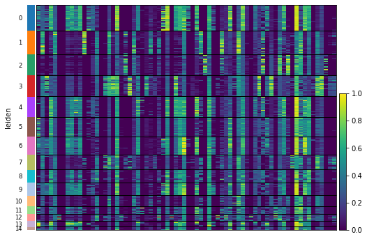
We perform aucell to compute the activity of each regulon on each spot.
[60]:
adata.X=adata.layers['x4']
SpaGTL.aucell(adata, normalize=True)
SpaGTL.heatmap_aucell(adata, adata.obsm['aucell'].columns, groupby='leiden')
100%|█████████████████████████████████████████████████████████████████████████████████| 72/72 [00:00<00:00, 117.77it/s]
WARNING: Gene labels are not shown when more than 50 genes are visualized. To show gene labels set `show_gene_labels=True`
We create a new object adata_aucell using the aucell matrix for visualization.
[61]:
adata_aucell = sc.AnnData(adata.obsm['aucell'])
adata_aucell.obs = adata.obs.copy()
adata_aucell.obsm = adata.obsm.copy()
adata_aucell.uns['spatial'] = adata.uns['spatial'].copy()
Finding differentially activity regulons#
We find the differentially activity regulons across identified domains and show the domains and their differentially activity regulons patterns in spatial coordinates.
[62]:
sc.tl.rank_genes_groups(adata_aucell, groupby='leiden', method='t-test_overestim_var')
[63]:
pd.DataFrame(adata_aucell.uns['rank_genes_groups']['names']).iloc[:10,:]
[63]:
| 0 | 1 | 2 | 3 | 4 | 5 | 6 | 7 | 8 | 9 | 10 | 11 | 12 | 13 | 14 | |
|---|---|---|---|---|---|---|---|---|---|---|---|---|---|---|---|
| 0 | Mef2c(+) | Ets2(+) | Sox10(+) | Zic1(+) | Tbx15(+) | Anxa11(+) | Nfib(+) | Tcf7l2(+) | Tbx15(+) | Nfib(+) | Pitx2(+) | Six3(+) | Hmgb2(+) | Anxa11(+) | Neurod2(+) |
| 1 | Elk1(+) | Nkx2-4(+) | Six6(+) | Shox2(+) | Nkx2-1(+) | Sebox(+) | Tbr1(+) | Lhx9(+) | Foxc1(+) | Pou3f1(+) | Isl1(+) | Otx2(+) | Foxc2(+) | Egr1(+) | Pou3f1(+) |
| 2 | Hlf(+) | Otp(+) | Nmral1(+) | Gbx2(+) | Foxc1(+) | Bhlhe22(+) | Jun(+) | Sox14(+) | Bhlhe22(+) | Tbr1(+) | Sp9(+) | Sp9(+) | Otx2(+) | Ovol2(+) | Sp8(+) |
| 3 | Pou3f1(+) | Pitx2(+) | Hnf1b(+) | Rora(+) | Bhlhe22(+) | Egr1(+) | Nkx2-1(+) | Gata3(+) | Rxrg(+) | Mafa(+) | Tcf7l2(+) | Lmx1a(+) | Tbx3(+) | Sebox(+) | Tbr1(+) |
| 4 | Foxc1(+) | Lhx6(+) | Hmgb2(+) | Lef1(+) | Egr4(+) | Egr3(+) | Nr4a3(+) | Zic4(+) | Egr3(+) | Mef2c(+) | Foxc2(+) | Nkx2-1(+) | Lmx1a(+) | Bhlhe22(+) | Hlf(+) |
| 5 | Ovol2(+) | Barhl1(+) | Sp9(+) | Irx2(+) | Smad3(+) | Ovol2(+) | Neurod2(+) | Zic5(+) | Neurod2(+) | Hlf(+) | Sox10(+) | Junb(+) | Six6(+) | Egr4(+) | Bhlhe22(+) |
| 6 | Tbr1(+) | Isl1(+) | Zic3(+) | Zic4(+) | Neurod1(+) | Neurod2(+) | Elk1(+) | Pitx2(+) | Mef2c(+) | Neurod2(+) | Gata3(+) | Nkx2-4(+) | Rax(+) | Elk1(+) | Mef2c(+) |
| 7 | Nfkb2(+) | Bsx(+) | Isl1(+) | Tcf7l2(+) | Sp8(+) | Tbx15(+) | Sp8(+) | Foxp2(+) | Foxc2(+) | Bcl11a(+) | Pbx3(+) | Rfx3(+) | Nkx2-4(+) | Egr3(+) | Elk1(+) |
| 8 | Egr3(+) | Gata3(+) | Rxrg(+) | Bcl11a(+) | Nr4a3(+) | Sp9(+) | Pou3f1(+) | Irx2(+) | Rfx3(+) | Sp8(+) | Lhx6(+) | Tbx15(+) | Six3(+) | Neurod2(+) | Smad3(+) |
| 9 | Mafa(+) | Lmx1a(+) | Foxc2(+) | Gata3(+) | Jun(+) | Smad3(+) | Ovol2(+) | Gbx2(+) | Smad3(+) | Elk1(+) | Shox2(+) | Anxa11(+) | Cebpb(+) | Smad3(+) | Foxc2(+) |
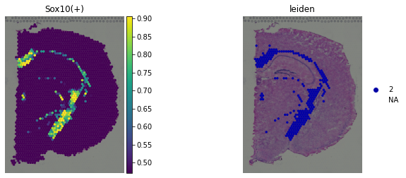
[110]:
sc.pl.spatial(
    adata_aucell,
    img_key='hires',
    color=['Sox10(+)','leiden'],
    frameon=False,
    alpha_img=1,
    size=1.65,
    palette=color,
    colorbar_loc='right',
    vmin='p90',
    vmax='p99',
    show=False,
    groups=[2]
)
[110]:
[<AxesSubplot: title={'center': 'Sox10(+)'}, xlabel='spatial1', ylabel='spatial2'>,
 <AxesSubplot: title={'center': 'leiden'}, xlabel='spatial1', ylabel='spatial2'>]
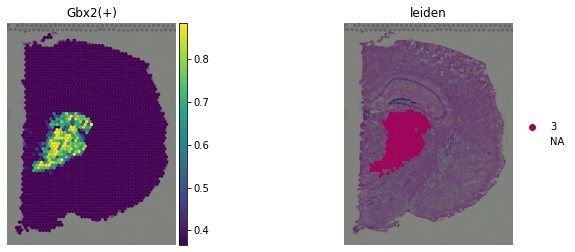
[108]:
sc.pl.spatial(
    adata_aucell,
    img_key='hires',
    color=['Gbx2(+)','leiden'],
    frameon=False,
    alpha_img=1,
    size=1.65,
    palette=color,
    colorbar_loc='right',
    vmin='p90',
    vmax='p99',
    show=False,
    groups=[3]
)
[108]:
[<AxesSubplot: title={'center': 'Gbx2(+)'}, xlabel='spatial1', ylabel='spatial2'>,
 <AxesSubplot: title={'center': 'leiden'}, xlabel='spatial1', ylabel='spatial2'>]